Wednesday, January 28, 2015

Food Waste Delusions


A couple months ago the New York Times convened a conference "Food for Tomorrow: Farm Better. Eat Better. Feed the World."  Keynotes predictably included Mark Bittman and Michael Pollan.  It featured many food movement activists, famous chefs, and a whole lot of journalists. Folks talked about how we need to farm more sustainably, waste less food, eat more healthfully and get policies in place that stop subsidizing unhealthy food and instead subsidize healthy food like broccoli.

Sounds good, yes? If you're reading this, I gather you're familiar with the usual refrain of the food movement.  They rail against GMOs, large farms, processed foods, horrid conditions in confined livestock operations, and so on.  They rally in favor of small local farms who grow food organically, free-range antibiotic free livestock, diversified farms, etc.  These are yuppies who, like me, like to shop at Whole Foods and frequent farmers' markets.  

This has been a remarkably successful movement.  I love how easy it has become to find healthy good eats, bread with whole grains and less sugar, and the incredible variety and quality of fresh herbs, fruits, vegetables and meat.  Whole Paycheck Foods Market has proliferated and profited wildly.  Even Walmart is getting into the organic business, putting some competitive pressure on Whole Foods. (Shhhh! --organic isn't necessarily what people might think it is.)

This is all great stuff for rich people like us. And, of course, profits.  It's good for Bittman's and Pollan's book sales and speaking engagements.  But is any of this really helping to change the way food is produced and consumed by the world's 99%?  Is it making the world greener or more sustainable?  Will any of it help to feed the world in the face of climate change?

Um, no.  

Sadly, there were few experts in attendance that could shed scientific or pragmatic light on the issues.  And not a single economist or true policy wonk in sight. Come on guys, couldn't you have at least invited Ezra Klein or Brad Plummer?  These foodie journalists at least have some sense of incentives and policy. Better, of course, would be to have some real agricultural economists who actually know something about large-scale food production and policies around the world. Yeah, I know: BORING!

About agricultural polices: there are a lot of really bad ones, and replacing them with good policies might help.  But a lot less than you might think from listening to foodies.  And, um, we do subsidize broccoli and other vegetables, fruits, and nuts.  Just look at the water projects in the West. 

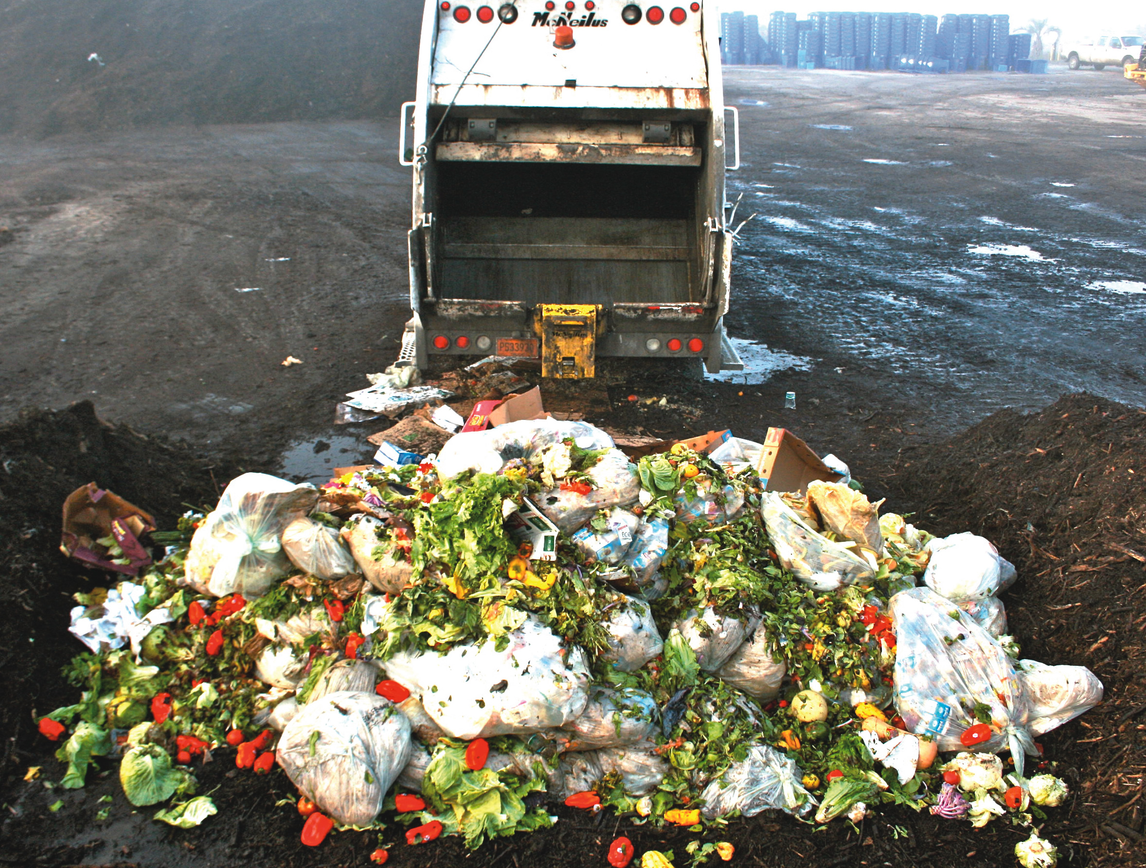
Let me briefly take on one issue du jour: food waste.  We throw away a heck of a lot of food in this country, even more than in other developed countries.  Why?  I'd argue that it's because food is incredibly cheap in this country relative to our incomes.  We are the world's bread basket.  No place can match California productivity in fruit, vegetables and nuts.  And no place can match the Midwest's productivity in grains and legumes.  All of this comes from remarkable coincidence of climate, geography and soils, combined with sophisticated technology and gigantic (subsidized) canal and irrigation systems in the West.  

Oh, we're fairly rich too.  

Put these two things together and, despite our waste, we consume more while spending less on food than any other country.  Isn't that a good thing?  Europeans presumably waste (a little) less because food is more scarce there, so people are more careful and less picky about what they eat. Maybe it isn't a coincidence that they're skinnier, too.

What to do? 

First, it's important to realize that there are benefits to food waste.  It basically means we get to eat very high quality food and can almost always find what we want where and when we want it.  That quality and convenience comes at a cost of waste.  That's what people are willing to pay for.  

If anything, the foodism probably accentuates preference for high quality, which in turn probably increases waste.  The food I see Mark Bittman prepare is absolutely lovely, and that's what I want.  Don't you?

Second, let's suppose we implemented a policy that would somehow eliminate a large portion of the waste.  What would happen?  Well, this would increase the supply of food even more.  And sinse we have so much already, and demand for food is very inelastic, prices would fall even lower than they are already.  And the temptation to substitute toward higher quality--and thus waste more food--would be greater still.  

Could the right policies help?  Well, maybe.  A little. The important thing here is to have a goal besides simply eliminating waste.  Waste itself isn't problem. It's not an externality like pollution.  That goal might be providing food for homeless or low income families.  Modest incentive payments plus tax breaks might entice more restaurants, grocery stores and others to give food that might be thrown out to people would benefit from it.  This kind of thing happens already and it probably could be done on a larger scale. Even so, we're still going to have a lot of waste, and that's not all bad. 

What about correcting the bad policies already in place?  Well, water projects in the West are mainly sunk costs.  That happened a long time ago, and water rights, as twisted as they may be, are more or less cemented in the complex legal history.   Today, traditional commodity program support mostly takes the form of subsidized crop insurance, which is likely causing some problems.  The biggest distortions could likely be corrected with simple, thoughtful policy tweaks, like charging higher insurance premiums to farmers who plant corn after corn instead of corn after soybeans.  But mostly it just hands cash (unjustly, perhaps) to farmers and landowners.  The odds that politicians will stop handing cash to farmers is about as likely as Senator James Inhofe embracing a huge carbon tax.  Not gonna happen.

But don't worry too much.  If food really does get scarce and prices spike, waste will diminish, because poorer hungry people will be less picky about what they eat.

Sorry for being so hard on the foodies.  While hearts and forks are in the right places, obviously I think most everything they say and write is naive.  Still, I think the movement might actually do some good.  I like to see people interested in food and paying more attention to agriculture.  Of course I like all the good eats.  And I think there are some almost reasonable things being said about what's healthy and not (sugar and too much red meat are bad), even if what's healthy has little to do with any coherent strategy for improving environmental quality or feeding the world.  

But perhaps the way to change things is to first get everyones' attention, and I think foodies are doing that better than I ever could.

Saturday, January 17, 2015

The Hottest Year Ever Recorded, But Not in the Corn Belt

Here's Justin Gillis in his usual fine reporting of climate issues, and the map below from NOAA, via the New York Times.


Note the "warming hole" over the Eastern U.S., especially the upper Midwest, the all important corn belt region.  We had a bumper crop this year, and that's because while most of the world was remarkably warm, the corn belt was remarkably cool, especially in summer.

Should we expect the good fortune to continue?  I honestly don't know...

Monday, January 12, 2015

Growth Effects, Climate Policy, and the Social Cost of Carbon (Guest post by Fran Moore)


Thanks to my thesis advisor (David) for this opportunity to write a guest post about a paper published today in Nature Climate Change by myself and my colleague at Stanford, Delavane Diaz. G-FEED readers might be familiar with a number of new empirical studies suggesting that climate change might affect not just economic output in a particular year, but the ability of the economy to grow. Two studies (here and here) find connections between higher temperatures and slower economic growth in poorer countries and Sol has a recent paper showing big effects of tropical cyclones on growth rates. Delavane and I simply take one of these empirical estimates and incorporate it into Nordhaus’ well-known DICE integrated assessment model (IAM) to see how optimal climate policy changes if growth-rates are affected by climate change.

The figure below shows why these growth effects are likely to be critical for climate policy. If a temperature shock (left) affects output, then there is a negative effect that year, but the economy rebounds the following year to produce no long-term effect. If growth rates are affected though, there is no rebound after the temperature shock and the economy is permanently smaller than it would otherwise be. So if temperature permanently increases (right), impacts to the growth rate accumulate over time to give very large impacts.


No IAMs so far have incorporated climate change impacts to economic growth. Of the three models used by the EPA to determine the social cost of carbon, two (PAGE and FUND) have completely exogenous growth rates. DICE is slightly more complicated because capital stocks are determined endogenously by the savings rate in the model. But any climate impacts on growth rates are very very small and indirect, so DICE growth rates are effectively exogenous.

We take the 2012 estimate by Dell, Jones and Olken (DJO) as our starting point and modify DICE in order to try and accurately incorporate their findings. We needed to make three major changes: firstly we split the global DICE model into two regions to represent developed and developing regions because DJO find big growth effects in poor countries but only modest effects in rich; secondly, we allowed temperature to directly affect growth rates by affecting either the growth in total factor productivity or the depreciation of capital, calibrating the model to DJO; and finally, since DJO estimates are the short-run impact of weather fluctuations, we explicitly allow for adaptation in order to get the response to long-term climate change (making some fairly optimistic assumptions about how quick and effective adaptation will be).

The headline result is given in the graph below that shows the welfare-maximizing emissions trajectory for our growth-effects model (blue) and for our two-region version of the standard DICE model (red). DICE-2R shows the classic “climate policy ramp” where mitigation is increased only very gradually, allowing emissions to peak around 2050 and warming of over 3°C by 2100. But our growth-effects model gives an optimal mitigation pathway that eliminates emissions in the very near future in order to stabilize global temperatures well below 2°C.


I think its worth just pointing out how difficult it is to get a model based on DICE to give a result like this. The “climate policy ramp” feature of DICE output is remarkably stable – lots of researchers have poked and prodded the various components of DICE without much result. Until now, the most widely discussed ways of getting DICE to recommend such rapid mitigation was either using a very low discount rate (a la Stern) or hypothetical, catastrophic damages at high temperatures (a la Weitzman). One of the main reasons I think our result is interesting is that it shows the climate policy ramp finding breaks down in the face of damages calibrated to empirical results at moderate temperatures, even including optimistic adaptation assumptions and standard discounting.

There are a bunch more analyses and some big caveats in the paper, but I won’t go into most of them here in the interests of space. One very important asterisk though is that the reason why poor countries are more sensitive to warming than rich countries has a critical impact on mitigation policy. If poorer countries are more vulnerable because they are poor (rather than because they are hot), then delaying mitigation to allow them time to develop could be better than rapid mitigation today. We show this question to be a big source of uncertainty and I think it’s an area where some empirical work to disentangle the effect of temperature and wealth in determining vulnerability could be pretty valuable.

I’ll just conclude with some quick thoughts that writing this paper has prompted about the connection between IAMs and the policy process. It does seem very surprising to me that these IAMs have been around for about 20 years and only now is the assumption of exogenous economic growth being questioned. Anyone with just a bit of intuition about how these models work would guess that growth-rate impacts would be hugely important (for instance, one of our reviewers called the results of this paper ‘obvious’), yet as far as I can tell the first paper to point out this sensitivity was just published in 2014 by Moyer et al.. This is not just an academic question because these models are used directly to inform the US government’s estimate of the social cost of carbon (SCC) and therefore to evaluate all kinds of climate and energy regulations. The EPA tried to capture possible uncertainties in its SCC report but didn’t include impacts to economic growth and so comes up with a distribution over the SCC that has to be too narrow: our estimate of the SCC in 2015 of $220 per ton CO2 is not only 6 times larger than the EPA’s preferred estimate of $37, but is almost twice the “worst case” estimate of $116 (based on the 95th percentile of the distribution). So clearly an important uncertainty has been missing, which seems a disservice both to climate impact science and to the policy process it seeks to inform. Hopefully that is starting to change.

So that’s the paper. Thanks again to the G-FEEDers for this opportunity and I’m happy to answer any questions in the comments or over email.
-Fran (fcmoore@stanford.edu)

Saturday, January 10, 2015

Searching for critical thresholds in temperature effects: some R code


If google scholar is any guide, my 2009 paper with Wolfram Schlenker on the nonlinear effects of temperature on crop outcomes has had more impact than anything else I've been involved with.

A funny thing about that paper: Many reference it, and often claim that they are using techniques that follow that paper.  But in the end, as far as I can tell, very few seem to actually have read through the finer details of that paper or try to implement the techniques in other settings.  Granted, people have done similar things that seem inspired by that paper, but not quite the same.  Either our explication was too ambiguous or people don't have the patience to fully carry out the technique, so they take shortcuts.  Here I'm going to try to make it easier for folks to do the real thing.

So, how does one go about estimating the relationship plotted in the graph above?

Here's the essential idea:  averaging temperatures over time or space can dilute or obscure the effect of extremes.  Still, we need to aggregate, because outcomes are not measured continuously over time and space.  In agriculture, we have annual yields at the county or larger geographic level.  So, there are two essential pieces: (1) estimating the full distribution of temperatures of exposure (crops, people, or whatever) and (2) fitting a curve through the whole distribution.

The first step involves constructing the distribution of weather. This was most of the hard work in that paper, but it has since become easier, in part because finely gridded daily weather is available (see PRISM) and in part because Wolfram has made some STATA code available.  Here I'm going to supplement Wolfram's code with a little bit of R code.  Maybe the other G-FEEDers can chime in and explain how to do this stuff more easily.

First step:  find some daily, gridded weather data.  The finer scale the better.  But keep in mind that data errors can cause serious attenuation bias.  For the lower 48 since 1981, the PRISM data above is very good.  Otherwise, you might have to do your own interpolation between weather stations.  If you do this, you'll want to take some care in dealing with moving weather stations, elevation and microclimatic variations.  Even better, cross-validate interpolation techniques by leaving one weather station out at a time and seeing how well the method works. Knowing the size of the measurement error can also help correcting bias.  Almost no one does this, probably because it's very time consuming... Again, be careful, as measurement error in weather data creates very serious problems (see here and here).

Second step:  estimate the distribution of temperatures over time and space from the gridded daily weather.  There are a few ways of doing this.  We've typically fit a sine curve between the minimum and maximum temperatures to approximate the time at each degree in each day in each grid, and then aggregate over grids in a county and over all days in the growing season.  Here are a couple R functions to help you do this:

# This function estimates time (in days) when temperature is
# between t0 and t1 using sine curve interpolation.  tMin and
# tMax are vectors of day minimum and maximum temperatures over
# range of interest.  The sum of time in the interval is returned.
# noGrids is number of grids in area aggregated, each of which 
# should have exactly the same number of days in tMin and tMax
 
days.in.range <- function( t0, t1 , tMin, tMax, noGrids )  {
  n <-  length(tMin)
  t0 <-  rep(t0, n)
  t1 <-  rep(t1, n)
  t0[t0 < tMin] <-  tMin[t0 < tMin]
  t1[t1 > tMax] <-  tMax[t1 > tMax]
  u <- function(z, ind) (z[ind] - tMin[ind])/(tMax[ind] - tMin[ind])  
  outside <-  t0 > tMax | t1 < tMin
  inside <-  !outside
  time.at.range <- ( 2/pi )*( asin(u(t1,inside)) - asin(u(t0,inside)) ) 
  return( sum(time.at.range)/noGrids ) 
}

# This function calculates all 1-degree temperature intervals for 
# a given row (fips-year combination).  Note that nested objects
# must be defined in the outer environment.
aFipsYear <- function(z){
  afips    = Trows$fips[z]
  ayear    = Trows$year[z]
  tempDat  = w[ w$fips == afips & w$year==ayear, ]
  Tvect = c()
  for ( k in 1:nT ) Tvect[k] = days.in.range(
              t0   = T[k]-0.5, 
              t1   = T[k]+0.5, 
              tMin = tempDat$tMin, 
              tMax = tempDat$tMax,
              noGrids = length( unique(tempDat$gridNumber) )
              )
  Tvect
}

The first function estimates time in a temperature interval using the sine curve method.  The second function calls the first function, looping through a bunch of 1-degree temperature intervals, defined outside the function.  A nice thing about R is that you can be sloppy and write functions like this that use objects defined outside of the environment. A nice thing about writing the function this way is that it's amenable to easy parallel processing (look up 'foreach' and 'doParallel' packages).

Here are the objects defined outside the second function:

w       # weather data that includes a "fips" county ID, "gridNumber", "tMin" and "tMax".
        #   rows of w span all days, fips, years and grids being aggregated
 
tempDat #  pulls the particular fips/year of w being aggregated.
Trows   # = expand.grid( fips.index, year.index ), rows span the aggregated data set
T       # a vector of integer temperatures.  I'm approximating the distribution with 
        #   the time in each degree in the index T

To build a dataset call the second function above for each fips-year in Trows and rbind the results.

Third step:  To estimate a smooth function through the whole distribution of temperatures, you simply need to choose your functional form, linearize it, and then cross-multiply the design matrix with the temperature distribution.  For example, suppose you want to fit a cubic polynomial and your temperature bins that run from from 0 to 45 C.  The design matrix would be:

D = [    0          0          0   
            1          1           1
            2          4           8
             ...
           45     2025    91125]

These days, you might want to do something fancier than a basic polynomial, say a spline. It's up to you.  I really like restricted cubic splines, although they can over smooth around sharp kinks, which we may have in this case. We have found piecewise linear works best for predicting out of sample (hence all of our references to degree days).  If you want something really flexible, just make D and identity matrix, which effectively becomes a dummy variable for each temperature bin (the step function in the figure).  Whatever you choose, you will have a (T x K) design matrix, with K being the number of parameters in your functional form and T=46 (in this case) temperature bins. 

To get your covariates for your regression, simply cross multiply D by your frequency distribution.  Here's a simple example with restricted cubic splines:


library(Hmisc)
DMat <- rcspline.eval(0:45)
XMat <- as.matrix(TemperatureData[,3:48])%*%DMat
fit <- lm(yield~XMat, data=regData)
summary(fit)

Note that regData has the crop outcomes.  Also note that we generally include other covariates, like total precipitation during the season,  county fixed effects, time trends, etc.  All of that is pretty standard.  I'm leaving that out to focus on the nonlinear temperature bit. 

Anyway, I think this is a cool and fairly simple technique, even if some of the data management can be cumbersome.  I hope more people use it instead of just fitting to shares of days with each maximum or mean temperature, which is what most people following our work tend to do.  

In the end, all of this detail probably doesn't make a huge difference for predictions.  But it can make estimates more precise, and confidence intervals stronger.  And I think that precision also helps in pinning down mechanisms.  For example, I think this precision helped us to figure out that VPD and associated drought was a key factor underlying observed effects of extreme heat.